IMPORTANT: This note is translated by LLM and fixed manually. See Chinese version for a more accurate note
1. Method of Lagrange Multipliers
1.1 Basic Definition
Lagrange first proposed the Method of Lagrange Multipliers for equality constraints.
Consider the following optimization problem:
$$ \begin{aligned} & \text{minimize} \quad & f_0(x)& \\\\ & \text{subject to} \quad & h_i(x) & = 0, \quad i=1, \cdots, m \end{aligned} $$Then we have the Lagrangian function:
$$ L(x, \nu) = f(x) + \sum_{i=0}^m \mu_i h_i(x) $$where $\mu$ is the Lagrange multiplier corresponding to each equality constraint. The formal expression of the Lagrangian function will be introduced later.
The general solution steps for the method of Lagrange multipliers are as follows:
- Construct the Lagrangian function
- Calculate the partial derivatives (gradient) of the Lagrangian function with respect to each variable, and set them to 0. This step does not require the function to be convex
- Solve the system of equations obtained in
2.to find the optimal point
The specific principle will be introduced in later sections
Thus, the method of Lagrange multipliers transforms the problem into an unconstrained optimization problem to some extent. The entire solution process does not need to consider the impact of constraint equations, as their effect has already been incorporated into the Lagrangian function.
1.2 Optimality Conditions
The necessary condition for optimality is that at the local optimal solution $x^\*$, the following must be satisfied:
1.2.1 Stationarity Condition
The optimal point must be a stationary point (of the Lagrangian function).
$$ \nabla_x L(x^\*, \mu^\*) = \nabla f(x^\*) + \sum_j \mu_j^\*\nabla h_j(x^\*)=0 $$Supplementary Concept: Stationary Point and Saddle Point
Stationary Point: For a function $\mathbb{R}^n\rightarrow \mathbb{R}$, if the gradient at point $x^\*$ is zero, i.e.:
$$ \nabla f(x^\*) = 0 $$then $x^\*$ is called a stationary point of function $f$.
When in some neighborhood of $x^\*$:
- If $f(x^\*) \geq f(x)$, then $x^\*$ is a local maximum point
- If $f(x^\*) \leq f(x)$, then $x^\*$ is a local minimum point
If neither of the above holds, then $x^\*$ is a saddle point of $f$. When $x^\*$ is a saddle point, it is not an optimal point.
1.2.2 Equality Constraints Satisfaction
$$ h_i(x^\*) = 0 $$1.3 Practical Examples
Note the following conditions for actual solving:
- The method of Lagrange multipliers cannot handle problems with inequality constraints; forcing equality will lead to inaccurate results
- All Lagrange multipliers themselves are also parameters to be solved, and should be treated equally with variable values
Example 1
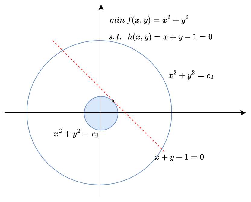
Its Lagrangian function is:
$$ L(x, y, \mu) = f(x, y) + \mu_1 h_1(x) = x^2+y^2 + \mu (x + y - 1) $$$$ h_1(x) = x+y-1=0 $$Calculate the partial derivatives of the Lagrangian function with respect to each variable
$$ \begin{cases} \frac{\partial L}{\partial x} = 2x+\mu = 0 \\\\ \frac{\partial L}{\partial y} = 2y + \mu = 0 \\\\ \frac{\partial L}{\partial \mu} = x+y-1 = 0 \end{cases} $$Solve this system of equations step by step:
$$ \begin{cases} 2x = -\mu \\\\ 2y = -\mu \\\\ x+y=1 \end{cases} $$$$ \begin{aligned} \mu &= -1\\\\ x &= \frac{1}{2} \\\\ y &= \frac{1}{2} \end{aligned} $$The usual order of solving is variables → Lagrange multipliers, prioritizing constraint equations
At this point, although $(x, y)$ is not a stationary point of the optimization objective, it is a stationary point of the problem’s Lagrangian function, being a stationary point while satisfying the constraints.
2. Lagrangian Function
Introducing inequality constraints to the method of Lagrange multipliers and further abstracting yields the Lagrangian function in the modern framework.
Consider the following optimization problem:
$$ \begin{aligned} & \text{minimize} \quad & f_0(x)& \\\\ & \text{subject to} \quad & g_i(x) &\leq 0, \quad i=1, \cdots, m \\\\ & & h_i(x) & = 0, \quad i=1, \cdots, p \end{aligned} $$Its Lagrangian function is defined as:
$$ L(x, \lambda, \mu) = f(x) + \sum_{i=1}^m \lambda_i g_i(x)+ \sum_{j=1}^p \mu_jh_j(x) $$where $\lambda_i$ is the Lagrange multiplier corresponding to the $i$-th inequality constraint ($g_i(x) \leq 0$), and $\mu_i$ is the Lagrange multiplier corresponding to the $i$-th equality constraint ($h_i(x)=0$). The vectors $\lambda$ and $\mu$ are called dual variables or the Lagrange multiplier vectors of the problem.
It can be seen that when there are no inequality constraints, the problem reduces to the Lagrangian function in the traditional multiplier method.
3. KKT Conditions (Karush-Kuhn-Tucker Conditions)
KKT conditions are conditions for determining optimal points of nonlinear optimization problems. In any case, KKT conditions are necessary conditions for optimal points, and when the problem is convex, they are necessary and sufficient conditions.
Note: Here it is assumed that the optimal point satisfies common constraint qualifications (CQ). Pathological problems do not satisfy CQ.
For whether it is convex and whether it satisfies CQ:
| Problem Type | Satisfies CQ (Non-pathological) | Necessity (Local Optimal → KKT) | Sufficiency (KKT → Local Optimal) |
|---|---|---|---|
| Convex Problem | ✓ | ✓ | ✓ |
| Convex Problem | ✗ | ✗ | ✓ |
| Non-convex Problem | ✓ | ✓ | ✗ |
| Non-convex Problem | ✗ | ✗ | ✗ |
KKT conditions include but are not limited to the two conditions in the method of Lagrange multipliers (stationarity condition, primal feasibility condition). Their complete formulation is as follows:
3.1 Stationarity Condition (First-order Condition)
$$ \nabla_x L(x^\* , \lambda^\*, \mu^\*) = 0 $$It can also be expressed as
$$ \nabla f(x^\*) + \sum_{i=1}^m \lambda_i^\* \nabla g_i(x^\*)+ \sum_{j=1}^p \mu_j^\*\nabla h_j(x^\*) = 0 $$The stationarity condition of KKT conditions is directly extended from the first-order condition definition of convex functions.
The solution of the method of Lagrange multipliers directly uses the necessity of this condition, that is, if an optimal solution exists, it must satisfy the system of equations with zero gradient (i.e., satisfies CQ).
3.2 Primal Feasibility Condition (Constraint Part)
That is, the optimal point must satisfy all constraints of the problem
$$ \begin{aligned} g_i(x) &\leq 0 \\\\ h_j(x) &= 0 \end{aligned} $$The method of Lagrange multipliers usually starts solving the system of equations from this part.
3.3 Dual Feasibility Condition
That is, the gradient direction of the function does not conflict with the optimization direction, meaning it does not damage the objective function.
$$ \lambda_i \geq 0 $$This condition is also directly related to shadow prices in economics, which will be introduced later.
For equality constraints, since they are two-sided, there is no inherent restriction on the direction of the gradient, and no additional consideration is needed during solving.
Concept Extension: Shadow Price
Shadow price, also known as optimal calculation price or calculation price, can reflect the true economic value of inputs and outputs, reflecting market supply and demand.
Consider the following resource optimization problem:
$$ \begin{aligned} \min \quad &f(x) \\\\ \text{s.t.} \quad & g_i(x) \leq b_i \quad \text{(Resource constraints)} \\\\ & h_j(x) = c_j \end{aligned} $$where $b_i$ can indicate a certain resource limit, such as the maximum power generation limit of a power plant.
This problem can have the following Lagrangian function:
$$ L(x, \lambda, \mu) = f(x) + \sum \lambda_i(b_i - g(x)) + \sum \mu_i (c_j - h(x)) $$During the solving process, calculating the Lagrange multipliers gives a shadow price, or it can be approximated as follows:
$$ \lambda_i^\* = \frac{\partial f^\*}{\partial b_i} \approx \frac{f^\*_{\text{new}} - f^\*}{\Delta b} $$That is, adding a small value $\Delta b$ to the right-hand side of the constraint to calculate the gradient. Here $f^\*_{\text{new}}$ needs to be recalculated.
Note:
- Accurate only when the constraint is linear and $\Delta b$ is small
3.4 Complementary Slackness Condition
$$ \lambda^\*_ig_i(x^\*) = 0 $$This feasibility is actually the intersection of the primal feasibility condition and dual feasibility condition in inequality constraints, that is, for inequality constraints, either the multiplier or the constraint must be zero
- When the constraint is active (tight): $g_i(x^\*)=0$, in this case the condition is satisfied regardless of the value of $\lambda_i$, and the constraint plays a limiting role
- When the constraint is inactive (slack): $g_i(x^\*) < 0$, in this case $\lambda_i = 0$ is required, meaning the constraint does not play an actual limiting role
4. Lagrangian Duality
4.1 Basic Definition
Consider the following optimization problem:
$$ \begin{aligned} & \text{minimize} \quad & f_0(x)& \\\\ & \text{subject to} \quad & g_i(x) &\leq 0, \quad i=1, \cdots, m \\\\ & & h_i(x) & = 0, \quad i=1, \cdots, p \end{aligned} $$From this we obtain its Lagrangian function
$$ L(x, \lambda, \mu) = f(x) + \sum_{i=1}^m \lambda_i g_i(x)+ \sum_{j=1}^p \mu_jh_j(x) $$The definition of its Lagrangian dual function is
$$ g(\lambda, \mu) = \inf_{x\in{\mathcal{D}}} L(x, \lambda, \mu) $$where $\inf$ denotes the infimum, and $\mathcal{D}$ is the domain satisfying the constraints.
Calculating the dual function can revolve around the “infimum” in the definition. Usually there are the following methods:
Take $L(x, \lambda) = x^2 + \lambda x + 1$ as an example
- Partial Derivative Method: Calculate partial derivatives with respect to independent variables to find extremum points. This method can only be used when the Lagrangian function is convex, but it is also the most stable method. Most kernels in SVM satisfy this condition.
- Inspection Method: Try to directly find extremum points, or transform the function into a form where extremum points can be visually identified, avoiding complex mechanical extremum point calculation. This method can only be applied to functions with simple structures such as quadratic functions, ReLU, etc.
Obviously, the minimum value can be achieved at $x=-\frac{\lambda}{2}$, and substituting gives the dual function.
Infimum
Let $S \subseteq \mathbb{R}$ be a non-empty set. If $\alpha$ is a lower bound of $S$ and $\alpha$ is the largest among them, then $\alpha$ is called the infimum of $S$.
The infimum is usually a point that can be approached infinitely but cannot be reached, such as 0 in $(0, 10]$, but it can also be a reachable point, such as 0 in $[0, 10]$.